Soil characteristics
Soil characteristics
Proof of their calculability
Numerous DIN and EN standards have been created according to various aspects for the identification, naming, classification, and loading of soils, e.g.:
DIN 1054 / EC/7, DIN 4020 up to DIN 4023, DIN 4030, DIN 18196, DIN 18300, DIN 19682-1+2, DIN 19682-2, DIN 19682-12, DIN EN 1997-1. DIN EN ISO 14688-1. DIN EN ISO 14688-2, DIN EN ISO 14689-1 and others.
In these standards, and based on magmatic, metamorphous or sedimentary primary rock, the soils are subdivided mainly according to grain shape, grain roughness, load-bearing capacity, and settling behaviour, as well as non-binding and binding soils. In general, the correspondingly derived soil characteristics are based on empirically found basic values. For earth pressure calculations, Prof. Dr. Rolf Katzenberg of the Institut und Versuchsanstalt für Geotechnik at the TU Darmstadt has summarized the enormous amount of Kagh values in tables, Fig. 1.
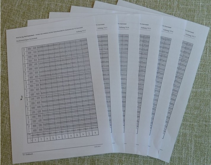
Fig. 1: Geotechnik study documents, TU Darmstadt – Annex VI-2 – Earth pressure of 10.03.2014
Regarding the tabulated values, it must be noted that at first sight they appear to be helpful for earth pressure calculations, but their negative influences are also revealed:
- All soil values are empiric, they have no direct reference to the soil type in question.
- The huge amount of tabulated values enables characteristics to be selected freely. This permits the use of values that provide a more favourable cost framework for the construction project.
- Likewise, in the event of a claim, the amount of tabulated values enables experts to freely attribute negligence to one party or the other, i.e. without any factual reference.
The new earth pressure teachings are based on the calculability of real soil properties and require no empiric random values. Own comprehensive laboratory investigations of dry, moist, and wet soils as well as soils under water revealed that every soil type exhibits distinctive properties. If soils are disturbed through natural or artificial interventions, new soil types are formed with own properties. Basis of the calculation method is the multiphase system of solid-state physics. The calculations are based on laboratory tests of extracted drill cores as well as undisturbed soil samples. All relevant values for earth pressure, load-bearing capacity, and settling behaviour of soils can be obtained from them.
Assumptions are made for calculating the soil properties, and the unit t/m³ soil is used for soil densities:
- The volume of soil mass is specified as Vp = 1.00 m³. Usually, this is divided into the solid body volume Vf and the pore volume Vl.
- Only the pore volume Vl can be partially or completely filled with liquid or water, whereby it is assumed that pore inclusions in the rock cannot take up any water, i.e. they remain dry.
- With wet soils, the pore volume changes from Vl to Vln.
- With moist soils, the water only partially fills pore volume Vl, whereby the water-filled volume Vl changes to volume Vli.
- Regarding density, hard rock/granite occupies the upper place in the soil scale, with density y90 = 29.42 kN/m³ equal to ptg90 = 3.0 t/m³ (ptg = new designation) with Vp = Vf = 1.00 m³;
- The lower place in the soil scale is occupied by primordial dust (new designation) with soil density ptg0 = 0.03 t/m³ with Vf = 0.01 m³;
- Density of the liquid/water pwg = 1.00 t/m³ (pwg = new designation).
Symbols are provided in the book „Die neue Erddrucklehre auf den reinen Grundlagen der Physik“.
The following values are determined under laboratory conditions from the extracted drill core and the undisturbed soil sample:
- Weight of undisturbed soil sample with known volume;
- Weight of the dried soil sample;
- Weight of the soil sample after complete filling with water;
- Adaptation of volume and the respective weighed weights to the volume Vp = 1.00 m³ result in the densities ptg (dry), pig (moist) and png (wet) with unit t /m³.
Comprehensive tests on soil behaviour have been conducted. They confirm the positions of inclination and shear planes of soils as shown in Figs. 2 and 3 (see own study).
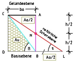
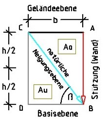
Fig. 2 shows the wedge areas Ao and Au, which are separated by the inclination plane with angle β.
Fig. 3 shows the ‚lying earth wedge‘ (C–L–D), the inclination plane, and the shear plane below angle s.
The following examples demonstrate that soil characteristics can be calculated:
Example 1: Calculated weight of dry soil mass F = 1.765 t, Fig. 4.
First, the soil density ptg with unit t / m³ is determined from the dry weight F of the soil sample, followed by solids volume Vf and pore volume Vl = Vli. Hereby, it is assumed that the total volume Vp is composed of Vp = Vf + Vl and pore volume Vl = Vlt with gas / air with density 0.0 t/m³. This dependency is used to calculate the solids volume Vf = F / ptg90 = 1.765 / 3.0 = 0.588 m³ and the pore volume Vp – Vf = 1.000 – 0.588 = 0.412 m³.
The inclination angle ßt can be calculated from the ratio Vli / Vf, tan ßt = Vf / Vli = 0.588 / 0.412 = 1.427 ⟶ ßt = 55.0°. The shear angle is formed by tan st = tan ßt /2 = 1.427 /2 = 0.714 ⟶ st = 35.5°.
The same result is obtained with the soil band (Fig. 4). Here, angle ßt is calculated using the volume ratio of the solid rock mass Vf90 = 1.00 m³ and the fictive pore volume Vl = h ∙ a ∙ ^b, whereby width ^b = Vl / = 0.412 / 0.588 = 0.70 m is represented. Or inclination angle tan ßt = h / ^b = 1.0 / 0.70 = 1.427 ⟶ ßt = 55.0°.
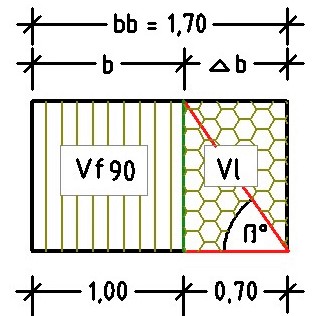
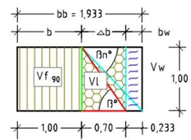
Fig. 4: Soil band without water content
Fig. 5: Soil band with water volume Vw
Example 2: Calculated weight of dry soil mass F = 1.765 t, and pore volume Vln = 0.412 m³, i.e. the pore volume has been filled completely with water (Fig. 5).
The addition of water (Fig. 5) increases the soil band’s weight (Fig. 4) to F‘ = Vf ∙ ptg90 + Vln ∙ pwg = 1.00 ∙ 3.0 + 0.70 ∙ 1.00 = 3.700 t. If this weight is standardized to the cube volume Vp = 1.00 m³, one obtains F” = F‘ ∙ b / (b + bw) = 3.70 ∙ 1.00 / (1.70) = 2.176 t. The soil cube can be used to calculate the wet density png = Vf ∙ ptg90 + Vln ∙ pwg = 0.588 ∙ 3.00 + 0.412 ∙ 1.00 = 2.176 t/m³.
When calculating the angles, it must be taken into account that a wet soil slides faster than a dry soil, i.e. the wet soil’s inclination angle is reduced. Consequently, water volume Vw and its width bw must be calculated first. The water volume results from Vw = pwg ∙ (^b ∙ h ∙ a) / ptg90 = 1.0 ∙ (0.70 ∙ 1.0 ∙ 1.0) / 3.0 = 0.233 m³ and has a width of bw = 0.233 m.
The inclination angle is calculated from tan ßn = h /(^b + bw) = 1.0 / (0.70 + 0.233) = 1.072 ⟶ ßn = 47.0°. The resulting shear angle is tan sn = tan ßn /2 = 1.072 /2 = 0.536 ⟶ shear angle sn = 28.2°.
Example 3: Calculated weight of dry soil mass F = 1.764 t (Fig. 4) plus measured water in the amount of 8% or water volume Vw = 80 liters per m³.
The absorbed water expands the dry soil band (Fig. 4) by volume Vli = (Vf + Vl) ∙ 8% = 1.70 ∙ 0.08 = 0.136 m³ or by the fictive width bw = Vli / h ∙ a = 0.136 / 1.0² = 0.136 m. Moreover, the water increases the soil band’s weight (Fig. 4) to F*= Vf ∙ ptg90 + Vli ∙ pwg = 1.00 ∙ 3.0 + 0.136 ∙ 1.00 = 3.136 t. Standardized to the cube volume Vp = 1.00 m³, this weight results in F* = F‘ ∙ b / (b + bw) = 3.136 ∙ 1.00 / (1.70) = 1.844 t, or alternatively in moist density pig = Vf ∙ ptg90 + Vli ∙ pwg = 0.588 ∙ 3.00 + 0.080 ∙ 1.00 = 1.844 t/m³.
As shown, the water changes the dry soil’s inclination angle ßt to the moist soil’s inclination angle ßi. The soil cube permits volume Vli = 0.080 m³ and thereby width bw = Vli / h ∙ a = 0.08 / 1.0 ∙ 1.0 = 0.08 m to be calculated. This leads to inclination angle ßi and shear angle si: tan ßi = Vf / (Vl + Vli / ptg90) = 0.588 / (0.412 + 0.080 /3) = 1.340 ⟶ ßi = 53.3° and shear angle tan si = tan ßi /2 = 1.340 /2 = 0.670 ⟶ si = 33.8°.
Example 4: Calculated weight of dry soil mass F = 1.764 t (Fig. 4) plus measured water Vw = 200 liters (20% moisture).
The example is intended to demonstrate the risk of a landslide that can arise from additional water absorption in the amount of 80 + 120 = 200 liters.
Soil properties are calculated from the soil cube Vp = 1.0 m³.
Water volume Vli = 0.08 + 0.120 = 0.200 m³, and width bw = Vli / h ∙ a = 0.20 / 1.0 ∙ 1.0 = 0.20 m. Moist density pig = Vf ∙ ptg90 + Vli ∙ pwg = 0.588 ∙ 3.00 + 0.20 ∙ 1.00 = 1.964 t/m³.
The moist soil’s inclination angle is calculated from: tan ßi = Vf / (Vl + Vli / ptg90) = 0.588 / (0.412 + 0.200 /3) = 1.228 ⟶ ßi = 49.4°.
The shear angle is given by tan si = tan ßi /2 = 1.228 / 2 = 0.614 ⟶ si = 31.5°.
Conclusion
With an embankment height of h = 10 m, the additional water absorbed by the soil shifts the slope base of the slightly moist soil (Example 3) by width bx = ho ∙ (tan 1.340 – tan 1.228) = 10 ∙ 0.112 = 1.12 m. The calculation example confirms that the new earth pressure teachings enable landslides to be calculated in advance.
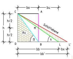
Fig. 6: Formation of the new plane C-L‘ caused by additional absorbance of water in the soil.